Bollinger Band for Beginners
Posted on August 17, 2022 by Quantplay Team ‐ 4 min read

A case study of bollinger bands -
Today, we are going to back-test bollinger bands over a period of three years using Quantplay. But before we get into that, Let us try to understand bollinger bands first.
What Is a Bollinger Band? -
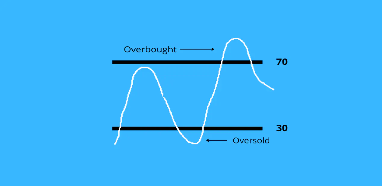
Bollinger Bands were developed and copyrighted by famous technical trader John Bollinger, designed to discover opportunities that give investors a higher probability of properly identifying when an asset is oversold or overbought.
This indicator is based on mean reversion model. Meaning, it says that whenever the price will hit the upper band it is more likely now, that the price will return back to its mean which is the middle band in this case and vise-versa.
Key details -
- There are three lines that compose Bollinger Bands
- A simple moving average (i.e middle band) and an upper and lower band
- The upper and lower bands are typically 2 standard deviations +/- from a 20-day SMA (simple moving average)
How to use bollinger bands in trading -
If the price is near the upper Bollinger Band, it’s considered “expensive” because it is 2 standard deviation above the average (the 20-period moving average). As a trader, we should sell here and expect the price to fall till it reaches the middle band.
If the is price near the lower Bollinger Band, it’s considered “cheap” because it’s 2 standard deviation below the average. We should buy here expecting the price to rise till it reacher the middle band.
Let’s test the strategy using quantplay’s library -
- Enter a trade at 9:20 AM (when the first 5-minute candle closes)
- Exit the trade at 3:15 PM or whenever the stoploss triggers
- Trade INR 1,00,000 in the stock
- Filter stocks that are outside of bollinger bands using Quantplay’s library
- Pick top 5 stocks based on the previous day performance
- Trade with a stop loss of 3%
Strategy Code -
from quantplay.strategy.base import QuantplayAlgorithm
from quantplay.utils.constant import TickInterval
from quantplay.service import market
import numpy as np
import pandas as pd
import ta

class BollingerBands(QuantplayAlgorithm):
    def __init__(self):
        self.interval = "5minute"
        self.entry_time = "09:15"
        self.exit_time = "15:15"
        self.exchange_to_trade_on = "NSE"
        self.stream_symbols_by_security_type = {"EQ": market.symbols(universe="FNO_STOCKS")}
        self.strategy_type = "intraday"
        self.strategy_tag = "bband"

        super(BollingerBands, self).__init__()

    def get_trades(self, market_data):
        trades = market.get_trades(market_data, self.entry_time)
        trades.loc[:, 'last_day_return'] = trades.close/trades.close.shift(1) - 1

        bbands = ta.volatility.BollingerBands(close=trades.close,
                                         window=20,
                                         window_dev=2)

        trades["bb_high"] = bbands.bollinger_hband()

        trades = trades[trades.close > trades.bb_high]
        trades = trades.sort_values("last_day_return", ascending=False).groupby(['date']).head(5)

        trades.loc[:, 'tradingsymbol'] = trades.symbol
        trades.loc[:, "transaction_type"] = "SELL"
        trades.loc[:, "stoploss"] = 0.02
        trades.loc[:, "quantity"] = (100000/trades.close).astype(int)

        return trades
strategy = BollingerBands()
strategy.validate()
res, trades = strategy.backtest()
Performance -
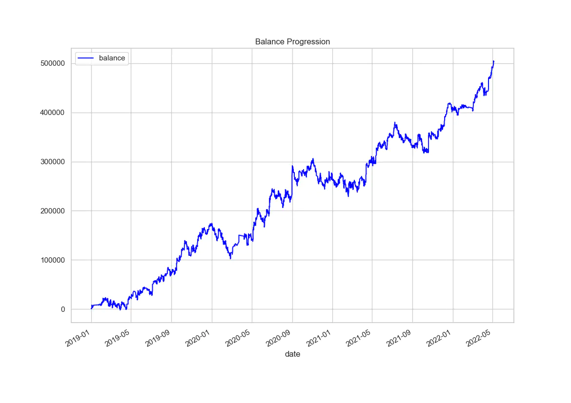
Fig: Balance progression from Jan-2019 till May-2022
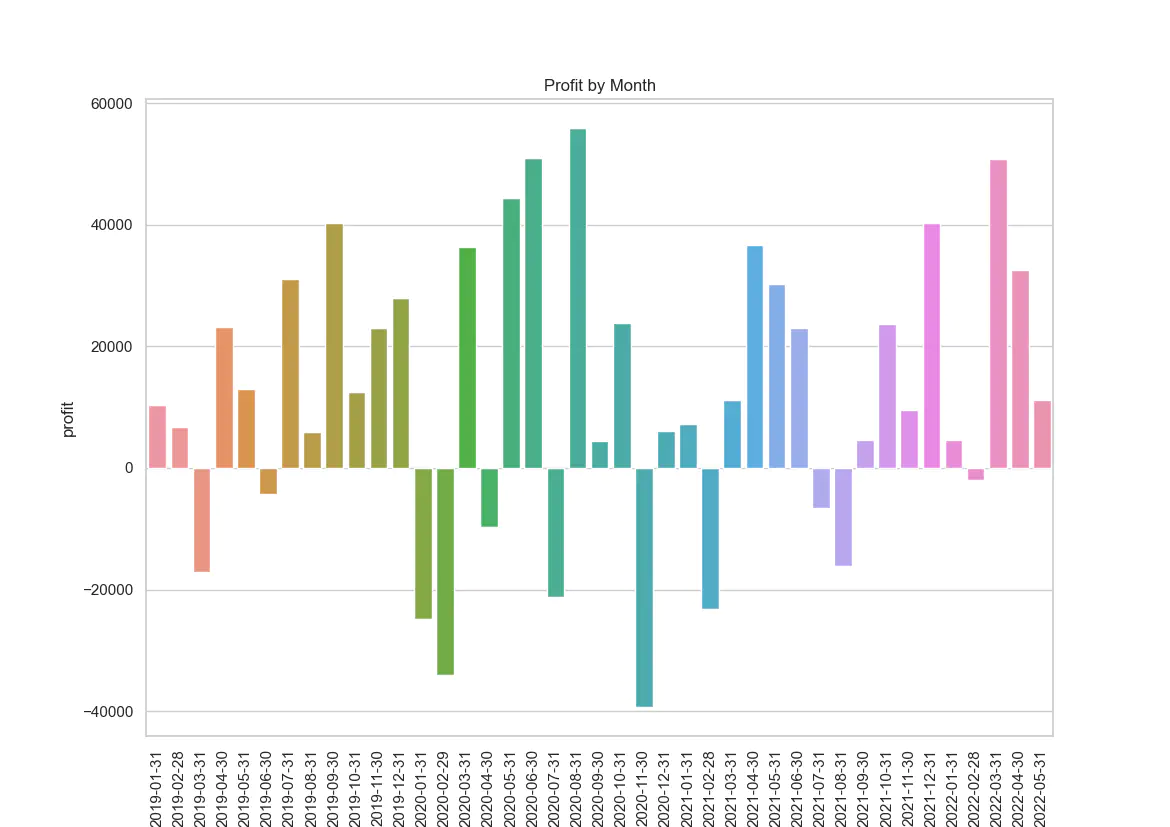
Fig: Profit gained on backtested data from 31st Jan 2019 till 31st May 2022
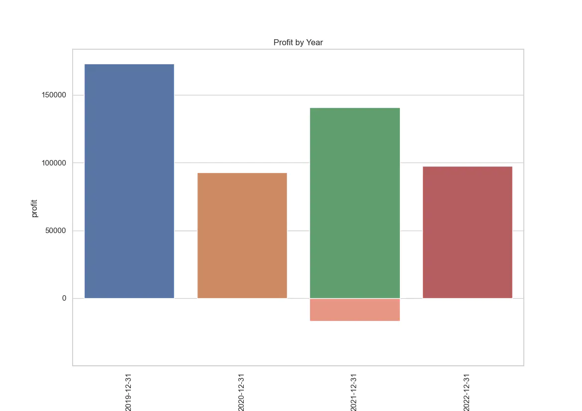
Fig: Profit gained on back-tested data from the year 2019 till till the year 2022
Strategy statistics -
| Attribute | Year 2019 | Year 2020 | Year 2021 | Year 2022 | All (Combining all the years) |
|---|---|---|---|---|---|
| Total profit | 173029 | 92725 | 140776 | 97345 | 5038745 |
| Max drawdown | 28575 | 71341 | 57578 | 25877 | 72393 |
| Sharpe ratio | 9.04 | 3.14 | 5.19 | 15.40 | 6.16 |
| Max drawdown days | 48 | 70 | 99 | 15 | 117 |
| Losing streak | 6 | 12 | 8 | 3 | 12 |
| Winning streak | 8 | 6 | 4 | 6 | 8 |
| Monthly pnl | 14419 | 7727 | 11731 | 19469 | 12290 |
| Required exposure | 100000 | 100000 | 100000 | 100000 | 100000 |
| Total signals | 964 | 1082 | 1132 | 305 | 3483 |
| Total trading days | 229 | 234 | 246 | 74 | 783 |
| Success ratio | 0.52 | 0.44 | 0.46 | 0.56 | 0.48 |
| Avg. pnl | 179 | 86 | 124 | 319 | 145 |
Conclusion -
Using only the bands to trade is a risky strategy since the indicator focuses on price and volatility, while ignoring a lot of other relevant information.In our upcoming blogs we are going to discuss the right market conditions to trade bands and improve the strategy results.
Follow us on your favorite social media to know when we post a better version of the strategy. You can now execute strategies like this using Quantplay library within seconds!
I hope you enjoyed reading this blog. Happy trading!
